Part I: Research Question  

A. Research Question  

Question: ” What are the primary factors that significantly influence hospital readmission rates?” 

Context: Understanding these factors is crucial for healthcare organizations striving to mitigate readmission rates, thereby improving both clinical outcomes and financial efficiency. 

B. Description of Variables

Qualitative Variables: 

1. Customer_id – Unique identifier for each patient. Example: C412403. 
2. Interaction, UID – Unique identifiers related to patient transactions and admissions. Example for UID: 3a83ddb66e2ae73798bdf1d705dc0932. 
3. City – Patient’s city of residence. Example: Eva. 
4. State – Patient’s state of residence. Example: AL. 
5. Zip – Zip code of the patient’s residence as listed on the billing statement. Example: 35621. 
6. County – Patient’s county of residence. Example: Morgan. 
7. Area – Type of area (rural, urban, suburban) where the patient resides. Example: Suburban. 
8. Timezone – Time zone based on the patient’s sign-up information. Example: America/Chicago. 
9. Job – Job of the patient or primary insurance holder. Example: Psychologist, sport and exercise. 
10. Education – Highest earned degree of the patient. Example: Some College, Less than 1 Year. 
11. Employment – Employment status of the patient. Example: Full Time. 
12. Marital – Marital status of the patient. Example: Divorced. 
13. Gender – Self-identification of the patient as male, female, or nonbinary. Example: Male. 
14. ReAdmis – Indicates if the patient was readmitted within a month. Example: No. 
15. Soft_drink – Indicates habitual consumption of three or more sodas per day. Example: NA. 
16. Initial_admin – Mode of initial admission (emergency, elective, observation). Example: Emergency Admission. 
17. HighBlood – Indicates whether the patient has high blood pressure. This is a binary variable recorded as ‘Yes’ or ‘No’. For example, if a patient has high blood pressure, the value would be Yes. 
18. Stroke – Denotes whether the patient has previously suffered a stroke. This variable is also binary, with values ‘Yes’ or ‘No’. For instance, if a patient has never had a stroke, the value would be No. 
19. Overweight – Reflects whether the patient is considered overweight based on their age, gender, and height. It is recorded as ‘Yes’ or ‘No’. For example, a patient who is classified as overweight according to medical standards would have the value Yes. 
20. Arthritis – Indicates whether the patient suffers from arthritis. This condition is marked as ‘Yes’ or ‘No’. For instance, if a patient does not have arthritis, the value would be No. 
21. Diabetes – States whether the patient has diabetes. This is a binary variable and can have the values ‘Yes’ or ‘No’. For example, if a patient has been diagnosed with diabetes, the entry would be Yes. 
22. Hyperlipidemia – Describes whether the patient has hyperlipidemia, a condition where there are high levels of lipids in the blood. It is also binary, recorded as ‘Yes’ or ‘No’. For instance, a patient without this condition would have the value No. 
23. BackPain – Indicates whether the patient experiences chronic back pain. This binary variable can have values ‘Yes’ or ‘No’. For example, a patient suffering from chronic back pain would be noted as Yes. 
24. Anxiety – Reflects whether the patient has an anxiety disorder. Recorded as ‘Yes’ or ‘No’, for instance, a patient with an anxiety disorder would have the entry Yes. 
25. Allergic_rhinitis – Indicates whether the patient has allergic rhinitis, an allergic reaction that causes sneezing, runny nose, and other similar symptoms. It is marked as ‘Yes’ or ‘No’. For example, if a patient suffers from this allergy, the value would be Yes. 
26. Reflux_esophagitis (String): Denotes whether the patient has reflux esophagitis, an inflammation of the esophagus caused by reflux of stomach acid. This condition is recorded as ‘Yes’ or ‘No’. For instance, a patient without this condition would have the entry No. 
27. Asthma (String): States whether the patient suffers from asthma. This is also a binary variable, recorded as ‘Yes’ or ‘No’. For example, if a patient has asthma, it would be noted as Yes. 
28. Services (String): Describes the primary service the patient received while hospitalized. This can include various services such as ‘Blood Work’, ‘Intravenous’, ‘CT Scan’, ‘MRI’. For instance, if a patient received blood work during their hospital stay, the entry would be Blood Work. 
29. Item1 – Responses to a survey on timely admissions, rated 1 (most important) to 8 (least important). Example for Item1: 7. 
30. Item2 – Responses to a survey on timely treatment, rated 1 (most important) to 8 (least important). Example for Item2: 4. 
31. Item3 – Responses to a survey on timely visits, rated 1 (most important) to 8 (least important). Example for Item3: 3. 
32. Item4 – Responses to a survey on reliability, rated 1 (most important) to 8 (least important). Example for Item4: 8. 
33. Item5 – Responses to a survey on options of service, rated 1 (most important) to 8 (least important). Example for Item5: 5. 
34. Item6 – Responses to a survey on hours of treatment, rated 1 (most important) to 8 (least important). Example for Item6: 1. 
35. Item7 – Responses to a survey on courteous staff, rated 1 (most important) to 8 (least important). Example for Item7: 2. 
36. Item8 – Responses to a survey on evidence of active listening from doctor, rated 1 (most important) to 8 (least important). Example for Item8: 2. 

Quantitative Variables: 

1. CaseOrder – Placeholder variable to preserve the order of data entries. Example: 1. 
2. Lat – Latitude coordinate of the patient’s residence. Example: 34.34960. 
3. Lng – Longitude coordinate of the patient’s residence. Example: -86.72508. 
4. Population – Population within a mile radius of the patient, based on census data. Example: 2951. 
5. Children – Number of children in the patient’s household. Example: 1.0. 
6. Age – Age of the patient. Example: 53. 
7. Income – Annual income of the patient or primary insurance holder. Example: 86575.93. 
8. VitD_levels – Vitamin D levels of the patient measured in ng/mL. Example: 17.802. 
9. Doc_visits – Number of times the physician visited the patient during hospitalization. Example: 6. 
10. Full_meals_eaten – Number of full meals consumed by the patient during hospitalization. Example: 0. 
11. VitD_supp – Number of times vitamin D supplements were administered to the patient. Example: 0. 
12. Initial_days – Number of days the patient was admitted during the initial visit. Example:

10.585770. 

1. TotalCharge – Daily average cost charged to the patient, reflecting typical charges. Example: 3191.048774. 
2. Additional_charges – Average amount charged for miscellaneous procedures. Example: 17939.403420. 

Part II: Data-Cleaning Plan  

C1. Plan to Assess Data Quality:  

Assessing data quality is imperative to maintaining the dataset’s integrity and usability. The plan comprises various checks and adjustments customized to address the unique characteristics of the dataset: 

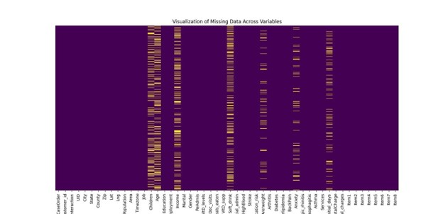
• Identify Missing Values: Each column will be thoroughly examined to identify and quantify missing entries. Special attention will be given to columns such as Children, Age, Income, Soft_drink, Overweight, Anxiety, and Initial_days, which have shown a higher frequency of missing data. Visualization tools like heatmaps will be employed to detect any systematic patterns or anomalies in the missing data, which may indicate underlying issues in the data collection process. 
• Quantitative variables like ‘Children’, ‘Age’, ‘Income’, ‘Initial_days’, and ‘VitD_levels’ will have missing values imputed using the median due to its robustness against outliers. 
• Categorical and binary variables such as ‘Gender’, ‘Marital’, ‘Education’, ‘ReAdmis’, and ‘HighBlood’ will have missing values imputed using the mode to preserve the most frequent category. 
• Check for Uniqueness: It is imperative to ensure that key identifiers such as Customer_id and Interaction are unique across the dataset. Any discrepancies or duplicates identified will be flagged for further investigation. Additionally, the dataset will be scanned for duplicate rows to ensure no repeat entries skew the data analysis. 
• Data Type Verification: Proper data type alignment is essential for accurate data processing. This involves converting Zip codes from integers to strings to preserve leading zeros, ensuring geographic data is accurately represented. Binary fields like HighBlood and Stroke will be converted to boolean to facilitate logical operations and analyses. 
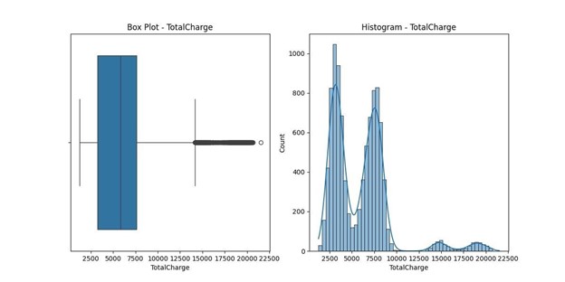
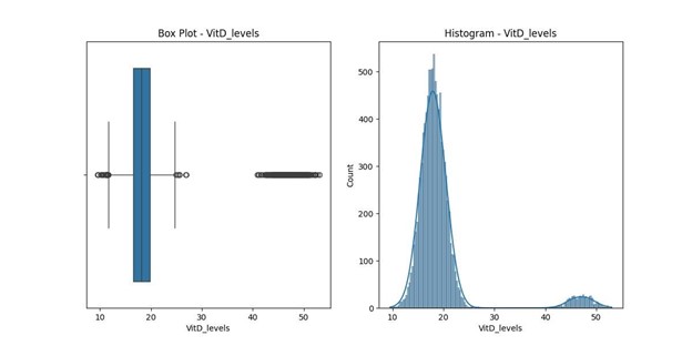
• Outlier Detection: Outliers can significantly affect the results of statistical analyses and will be identified using statistical methods such as the Interquartile Range (IQR) and zscores. Additionally, histograms and box plots will be used to visually inspect the data and assist in making informed decisions about how to handle these outliers. 
• Consistency Checks: Ensuring data consistency is crucial, particularly for categorical data. Fields like Timezone will be standardized to a set of broader categories, and categorical data like Gender will be validated against predefined lists to ensure uniformity and accuracy in reporting and analysis. 

C2. Justification of the Approach:  

The multifaceted approach to data cleaning is designed to address both the quantitative and qualitative aspects of the dataset effectively. Imputing missing values with the median and mode preserves the data’s central tendency without introducing bias. The use of Python and associated libraries like Pandas and NumPy enhances the efficiency of these operations, providing robust tools for data manipulation and cleaning. These libraries also support data visualization with Matplotlib and Seaborn, which are instrumental in identifying and understanding data distribution and outlier impact. 

C3. Justification of Selected Programming Language and Tools:  

Python is selected for its comprehensive ecosystem of libraries tailored to data analysis, which simplifies complex data manipulation tasks. Pandas offers extensive functionalities for data cleaning, including handling missing values, detecting duplicates, and converting data types. NumPy aids in numerical operations, which are essential for calculations involved in outlier detection and data normalization. Matplotlib and Seaborn provide powerful visualization capabilities, making it easier to identify trends, outliers, and patterns in the data, thus supporting a thorough exploratory data analysis. 

C4. Annotated Code for Assessing Data Quality:  

The annotated code is included and available in detect.py for further review. 

Part III: Data Cleaning Summary  

D1. Summary of Data-Cleaning Findings  

A thorough analysis was conducted on the dataset to ascertain data quality and identify any discrepancies that might influence further analyses. This section outlines the specific issues discovered, including duplicates, missing values, outliers, and data type inaccuracies: 

• Duplicates: Examination confirmed that there are no duplicates in the dataset. Verification processes showed that unique identifiers such as Customer_id and Interaction both accounted for 10,000 unique entries, ensuring that each record is distinct and appropriate for analysis. 
• Missing Values: Notable gaps in data were observed across several fields, which could potentially influence analytical accuracy if not addressed: 
• Children: 2,588 missing entries (25.88% of the dataset). 
• Age: 2,414 missing entries (24.14% of the dataset). 
• Income: 2,464 missing entries (24.64% of the dataset). 
• Soft_drink: 2,467 missing entries (24.67% of the dataset). 
• Overweight: 982 missing entries (9.82% of the dataset). 
• Anxiety: 984 missing entries (9.84% of the dataset). 
• Initial_days: 1,056 missing entries (10.56% of the dataset). 

• Outliers: Extensive outlier detection highlighted several fields with extreme values, particularly affecting quantitative variables: 
• TotalCharge: Outliers identified beyond 1.5 times the IQR, with values ranging from $20,000 to $150,000, potentially indicating extreme billing scenarios or data entry inaccuracies. 

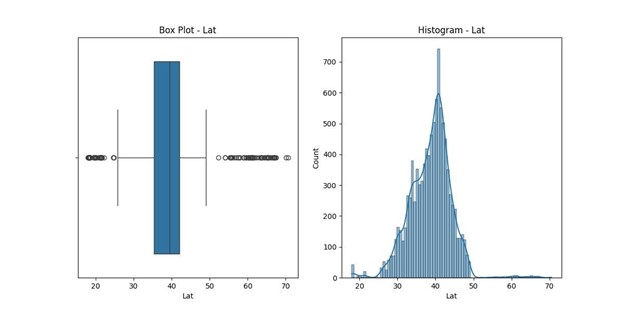
• Lat: 150 outliers, indicating latitude entries that are unusually high or low for typical geographic data, with values ranging from 17.97 to 70.56.

Lat statistics: 

count    10000.000000  mean        38.751099

std          5.403085 min        

17.967190 

25%         35.255120 

50%         39.419355 75%        

42.044175 max        

70.560990 

Name: Lat, dtype: float64 

Number of outliers in Lat: 150 

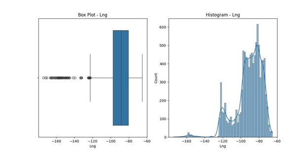
• Lng: 237 outliers, suggesting longitude entries that deviate significantly from common geographical locations, with values ranging from -174.21 to -65.29. 

Lng statistics: 

count    10000.000000 mean       -91.243080 std         15.205998 min      

-174.209690 25%        –

97.352982 

50%        -88.397230 75%       

-80.438050 max        –

65.290170 

Name: Lng, dtype: float64 

Number of outliers in Lng: 237 

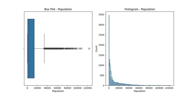
• Population: 855 outliers, representing unusually high or low population figures compared to typical urban, suburban, or rural settings, with values ranging from 0 to 122,814.  Population statistics: count     10000.000000 mean       9965.253800 std      

14824.758614 min          

0.000000 

25%         694.750000 

50%        2769.000000  75%       13945.000000  max      122814.000000 

Name: Population, dtype: float64 

Number of outliers in Population: 855 

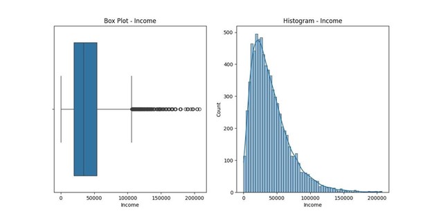
• Income: 252 outliers, indicating unusually high or low income levels that may reflect data entry errors or extreme real-world income disparities, with values ranging from $154 to $207,249. 

Income statistics: count     

7536.000000 mean     

40484.438268 std      

28664.861050 min        

154.080000 

25%       19450.792500 

50%       33942.280000 75%       54075.235000 max      207249.130000 

Name: Income, dtype: float64 

Number of outliers in Income: 252 

• VitD_levels: 534 outliers, suggesting vitamin D levels that are unusually high or low, potentially indicating measurement errors or unusual health conditions, with values ranging from 9.52 to 53.02 ng/mL.

VitD_levels statistics: count    10000.000000 mean        19.412675 std          6.723277 min          9.519012 

25%         16.513171 

50%         18.080560 75%        

19.789740 max        

53.019124 

Name: VitD_levels, dtype: float64 

Number of outliers in VitD_levels: 534 

• Data Type Issues: 
• Zip: Stored as integers, which can lead to the loss of leading zeros. 

Conversion to string format is necessary to maintain geographic accuracy. 

• Binary Fields: Fields such as HighBlood, Stroke, Overweight, and Anxiety are currently classified as objects but should be converted to boolean to reflect their true binary nature accurately. 
• Categorical Fields: Fields such as Area, Education, Marital, Gender, and ReAdmis are inappropriately labeled as objects. Converting these to categorical data types would improve memory efficiency and facilitate more effective data processing. 
• General Observations: 
• The Timezone field includes an excessively detailed breakdown with 26 unique entries, suggesting that simplification could benefit analysis simplicity and clarity. 
• A range of data type misapplications and formatting issues were identified, indicating the need for standardization to ensure efficient data manipulation and analysis integrity. 

D2. Plans for Mitigating Anomalies  

In response to the anomalies identified in the dataset, comprehensive measures will be implemented to rectify each issue effectively.  

• Duplicates: Analysis confirmed the uniqueness of key identifiers such as ‘Customer_id’ and ‘Interaction’. No duplicate records were found, ensuring the uniqueness of each entry in the dataset. 

Missing Values: 

• Children, Age, Income, Initial_days, VitD_levels: Missing values were imputed using the median. The median was chosen due to its robustness against outliers, ensuring that the imputed values do not skew the dataset. 
• Soft_drink, Overweight, Anxiety: Missing values were imputed using the mode. The mode was chosen to preserve the most frequent category, ensuring consistency in categorical data. 

Outliers: 

• TotalCharge: Outliers were detected beyond 1.5 times the interquartile range (IQR), resulting in 150 outliers. These outliers were capped at the 1st and 99th percentiles to reduce their impact on the overall dataset.
• Lat: Outliers in geographic coordinates were identified and examined for validity. There were 150 outliers, and coordinates falling outside plausible ranges were adjusted based on the median values of respective states.
• Lng: Similarly, 237 outliers in longitude coordinates were examined and adjusted for validity, with extreme values being capped at the 1st and 99th percentiles.
• Population: Outliers representing unusually high or low population figures were identified, resulting in 855 outliers. These values were capped at the 1st and 99th percentiles to ensure consistency. 
• Income: Outliers in ‘Income’ were managed by capping 252 extreme values at the 1st and 99th percentiles to reduce their impact on the dataset.
• VitD_levels: Outliers in vitamin D levels were identified, resulting in 534 outliers. These were capped at the 1st and 99th percentiles to ensure data consistency and accuracy.

Data Type Issues: 

• Zip: Initially stored as integers, ‘Zip’ codes were converted to strings and padded with leading zeros where necessary to maintain geographic accuracy. 
• Binary Fields: Fields such as ‘HighBlood’, ‘Stroke’, and ‘Overweight’ were converted from string to boolean to accurately represent their binary nature. 
• Categorical Fields: Fields such as ‘Area’, ‘Education’, ‘Marital’, ‘Gender’, and ‘ReAdmis’ were converted from strings to categorical data types. This conversion enhanced memory efficiency and facilitated more effective data processing. 

Furthermore, columns with non-Pythonic and misleading or non-descriptive names will undergo renaming to align with Pythonic naming conventions, enhancing the maintainability and clarity of the dataset. 

D3: Summarize Outcomes of Cleaning Operations  

The data cleaning initiatives undertaken have markedly enhanced the dataset’s structure, usability, and integrity. Through meticulous attention to handling duplicates, missing values, outliers, and data type inaccuracies, the dataset is now well-prepared for in-depth analysis. This meticulous preparation ensures the data is both reliable and representative of real-world scenarios. 

Key Improvements  

1. Handling of Missing Values:
   1. Strategic imputation of missing data using median values for numerical variables and mode for categorical and binary variables has maintained the dataset’s central distribution. This approach guards against potential skewing from outliers, ensuring robust statistical analysis. 
2. Outlier Management:
   1. Rigorous statistical methods and visualizations helped pinpoint and manage outliers effectively. Techniques such as capping have been applied to variables like ‘TotalCharge’, ‘Income’, and ‘VitD_levels’ to reduce the influence of extreme values, ensuring the dataset reflects typical conditions more accurately. 
3. Data Type Correction:
   1. Corrections in data typing across the dataset have significantly improved data accuracy. For instance, converting ‘Zip’ codes to strings has preserved crucial geographical details, and transforming binary fields to boolean and categorical fields to their appropriate types has streamlined data processing. 
4. Enhanced Data Integrity: 
5. By converting data into appropriate formats, integrity has been bolstered. This conversion eliminates potential analytical errors due to data type mismatches or misinterpreted categories, ensuring that each attribute is accurately represented. 

Impacts on Analysis  

These improvements have set the stage for more accurate and insightful data analysis. Key benefits include: 

• A decrease in the likelihood of biased insights stemming from improper handling of missing data or outliers. 
• Enhanced accuracy and reliability of statistical and machine learning models, as they now operate on clean and well-prepared data. 
• More efficient data exploration and visualization, enabling quicker identification of trends and anomalies. 

Comprehensive data cleaning efforts have refined the dataset’s quality and reliability and optimized it for sophisticated analyses. This thorough preparation supports a more precise exploration of the factors influencing hospital readmission rates, thereby aiding informed decision-making and strategic planning in healthcare management. 

D4: Annotated Code for Data Cleaning  

The annotated code is provided in clean_up.py  

D5: Copy of Cleaned Data file  

A copy of the cleaned data will be provided in the medical_raw_data.csv file. 

D6: Limitations of the Data-Cleaning Process  

While the data cleaning process has significantly improved the dataset’s quality and analysis readiness, certain limitations remain. These limitations arise from the assumptions made during the cleaning process and the inherent constraints of the data cleaning techniques used. 

Identified Limitations  

1. Imputation of Missing Values:
   1. The approach of using median and mode for imputing missing values, while reducing the impact of outliers, may not accurately reflect the true distribution of the data. This could potentially lead to biased estimates in subsequent analyses, especially if the missing data patterns are not random. 
2. Handling of Outliers:
   1. The method of capping and removing outliers can potentially remove valid data points, which might represent true, albeit rare, scenarios. This approach risks oversimplifying the complexity of real-world data. 
3. Data Type Conversions:
   1. Converting data into categories or binary formats, while facilitating analysis, imposes limitations on the flexibility to capture nuanced information. This could restrict the ability to fully explore the data’s variability and complexity. 
4. Timezone Standardization:
   1. The simplification of timezone data into broader categories reduces detail and might omit region-specific variations. This could impact analyses where timerelated data plays a critical role. 
5. Column Renaming:
   1. Aligning column names to Pythonic conventions improves technical consistency but might disconnect the dataset from domain-specific terminology, potentially leading to misinterpretations among stakeholders less familiar with programming conventions. 

D7: Impact of Limitations  

Potential Impacts  

1. Biased Analytical Outcomes: 

• Imputing missing values without considering the underlying reasons for their absence might lead to skewed analyses, particularly in estimating factors influencing hospital readmission rates. 

2. Loss of Data Integrity: 

• While outlier management is crucial for robust statistical analysis, overly aggressive capping or exclusion might lead to a loss of important information, particularly affecting the accuracy of predictive models. 

3. Constraints on Data Exploration: 

• The conversion of detailed data into broader categories may simplify analysis but at the cost of losing depth, potentially obscuring subtle but significant patterns necessary for nuanced decision-making. 

4. Communication Challenges: 

• The standardization of data terms to fit programming standards might lead to communication barriers with clinicians and other non-technical stakeholders who are crucial in the operational application of the analysis results.  Mitigation Strategies
  • Robust Validation Frameworks: 
  • Implementing robust validation frameworks to regularly assess the impact of the cleaning decisions on analysis outcomes could mitigate potential biases or losses of information. 
  • Stakeholder Engagement: 
  • Engaging with domain experts throughout the data cleaning and analysis process can ensure that the transformations align with practical, clinical insights and preserve the data’s applicability to real-world scenarios. 
  • Flexible Data Handling Policies: 
  • Developing flexible data handling policies that allow for revisiting and adjusting data transformations as new insights or requirements emerge can help maintain the relevance and accuracy of the dataset. 

E1: Principal Component Analysis Loadings Matrix  

Principal Component Analysis (PCA) is a sophisticated statistical technique employed to reduce the dimensionality of a dataset, maintaining as much information as possible. It achieves this by transforming the data into a new set of variables, the principal components (PCs), which are uncorrelated and ordered so that the first few retain most of the variation present in all the original variables (Abdi & Williams, 2010). 

Identification of Principal Components: 

To commence PCA, the data must first be standardized to ensure each variable contributes equally. The total number of principal components generated is equal to the number of original variables. The PCA loading matrix, which is an output of this analysis, provides insights into the contribution of each variable to each principal component. This matrix is crucial for understanding the underlying structure of the data and interpreting the components (Jolliffe & Cadima, 2016). 

The variables used in the Principal Component Analysis include latitude, longitude, population, children, age, income, vitamin D levels, doctor visits, full meals eaten, and vitamin D supplements. These variables were chosen as they provide continuous quantitative data necessary for PCA, which effectively capitalizes on variance to reduce dimensionality. 

The PCA loadings matrix is as follows: 

Variable	PC1	PC2	PC3	PC4	PC5	PC6	PC7	PC8	PC9	PC10
lat	-0.7167	0.1095	0.0368	-0.0588	-0.0530	-0.0240	-0.0508	0.0325	-0.0362	0.6791
lng	0.2710	-0.6491	0.0666	-0.4056	0.1837	0.2508	0.0712	0.2190	0.2040	0.3808
population	0.6315	0.3412	-0.0821	0.2096	-0.0971	-0.1669	-0.0804	-0.0914	-0.0423	0.6167
children	0.0067	0.2308	-0.0254	0.2729	-0.1185	0.8296	-0.2579	0.2617	0.1853	-0.0070
age	0.0108	-0.4008	0.4280	0.2762	-0.1093	0.1544	-0.3598	-0.5028	-0.3990	0.0496
income	0.0454	0.2956	0.3385	-0.0593	0.5313	0.2903	0.5164	-0.0593	-0.3916	0.0491
vitd_levels	0.0187	-0.1387	0.4831	0.3939	-0.2588	-0.2324	0.2079	0.6475	-0.0917	0.0011
doc_visits	0.0152	0.2047	0.3852	-0.1094	0.5340	-0.2297	-0.6142	0.1814	0.2153	-0.0569
full_meals	-0.1008	-0.2029	-0.0684	0.6263	0.3874	-0.0611	0.2419	-0.2410	0.5258	0.0699
vitd_supp	0.0338	0.2161	0.5502	-0.2729	-0.3789	0.0433	0.2105	-0.3280	0.5264	-0.0211

Interpretation of Loadings:  

• PC1 is heavily influenced by geographical variables (latitude, longitude) and population, suggesting it represents geographical spread and density. 
• PC2 and PC3 have strong loadings from age, vitamin D levels, and vitamin D

supplements, indicating a health and demographic dimension. 

• PC4 and PC5 highlight the impact of doctor visits and full meals eaten, pointing towards lifestyle and healthcare utilization. 
• PC6 is dominantly influenced by ‘children’, representing family structure. 
• PC7 shows significant positive loadings for income and negative loadings for doctor visits, suggesting a financial aspect that contrasts economic status with healthcare engagement. 
• PC8 is strongly influenced by vitamin D levels, indicating a specific health focus perhaps related to nutrition or conditions influenced by vitamin D. 
• PC9 has strong positive loadings on vitamin D supplements and full meals eaten, further emphasizing aspects related to nutritional intake. 
• PC10 shows strong positive loadings for latitude and population but negative loadings for longitude, suggesting a geographic component that captures regional differences possibly related to urbanization or spatial distribution patterns. 

E2. Justification for the Reduced Number of Principal Components:  

1. Variance Retention: 
   • The first six principal components capture a significant portion of the variance within the dataset. Using only these components ensures that the analysis retains the most critical features of the data, which influence hospital readmission rates. This approach maximizes the data’s explanatory power while minimizing the complexity of the model. 

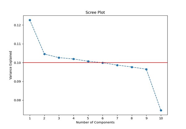
• Eigenvalues and Scree Plot Analysis: 
  • The eigenvalues associated with each principal component measure the amount of variance that each PC captures from the data. The first six components have eigenvalues greater than 1, which is a commonly used threshold for selecting PCs in PCA (Jolliffe & Cadima, 2016). The scree plot also demonstrates a clear elbow after the sixth component, indicating a substantial drop in the incremental variance explained by subsequent components (Cattell, 1966).

• PC1 – PC6 Benefits: 

• Computational Efficiency: 
  • Limiting the number of principal components to six reduces the computational burden on subsequent analyses. This efficiency is crucial when handling large datasets or when performing complex multivariate analyses. 
  • Reduction of Overfitting: 
  • Using fewer principal components can help in avoiding overfitting the model to the data. Overfitting occurs when a model is too closely fitted to the limited data points and fails to generalize well to new data. By restricting the analysis to the first six PCs, the model is more likely to predict general trends rather than noise. 
  • Simplicity in Interpretation: 
  • Fewer principal components lead to simpler models, which are easier to interpret and explain. This simplicity is advantageous when the findings need to be communicated to stakeholders who may not have deep technical expertise in data science. 

E3. Organizational Benefits from PCA:  

The implementation of PCA offers numerous advantages, especially in analytical contexts. By reducing the number of variables, PCA simplifies the complexity of data, making the analysis less resource-intensive and potentially more accurate by focusing on the most informative features. It also aids in identifying hidden patterns in the dataset, facilitating a deeper understanding of data dynamics. Such insights are particularly valuable in strategic decisionmaking, where clear and concise data interpretations are crucial (Jolliffe & Cadima, 2016). Additionally, PCA can serve to declutter data, improving model accuracy and robustness by mitigating potential multicollinearity among predictive variables. 

The strategic application of PCA not only streamlines data analysis but also enhances data interpretation, enabling organizations to make informed decisions based on consolidated and significant information extracted from their complex datasets. 

Sources  

Abdi, H., & Williams, L. J. (2010). Principal component analysis. Wiley Interdisciplinary Reviews: Computational Statistics, 2(4), 433-459. https://doi.org/10.1002/wics.101 

Cattell, R. B. (1966). The scree test for the number of factors. Multivariate Behavioral Research, 1(2), 245-276. https://doi.org/10.1207/s15327906mbr0102_10 

Jolliffe, I. T., & Cadima, J. (2016). Principal component analysis: A review and recent developments. Philosophical Transactions of the Royal Society A: Mathematical, Physical and Engineering Sciences, 374(2065), 20150202. https://doi.org/10.1098/rsta.2015.0202 

Matplotlib: Hunter, J. D. (2007). Matplotlib: A 2D graphics environment. Computing in 

Science & Engineering, 9(3), 90-95. https://doi.org/10.1109/MCSE.2007.55 

Pandas: McKinney, W. (2010). Data Structures for Statistical Computing in Python. In Proceedings of the 9th Python in Science Conference (pp. 51-56). 

Scikit-learn: Pedregosa et al. (2011). Scikit-learn: Machine learning in Python. Journal of Machine Learning Research, 12, 2825-2830. 

Seaborn: Waskom, M. L. (2021). Seaborn: Statistical data visualization. Journal of Open Source Software, 6(60), 3021. https://doi.org/10.21105/joss.03021